Customer Anomaly DetectionMachine Learning
Finding the customers whose behaviour doesn't add up, in a telco's data. My slice of a four-person team project.
Each of four team members owned one model family over a telco dataset; mine was anomaly detection, plus the usage-data cleaning everyone built on. Across 7,043 customers the flagged group was not single outliers but combinations of extremes, with ten times the refunds and thirteen times the extra data charges, reading as refund abuse, referral fraud or missed upsells.
My slice: usage data and anomalies
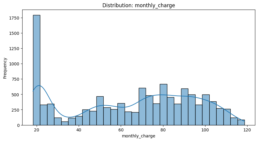
The scenario is a telecom company opening its customer data to a new data science team, one ML task per department: revenue forecasting, churn, segmentation, and mine, abnormal behaviour for the risk team. I also owned the usage dataset itself: 11,125 rows with a quarter of revenue values missing, rebuilt from the billing identity (charges plus extras minus refunds) instead of blanket imputation. The EDA surfaced a pricing gap on the way: customers cluster at the minimum plan or above 50 dollars, with almost nobody in between.
Designing an unsupervised evaluation honestly
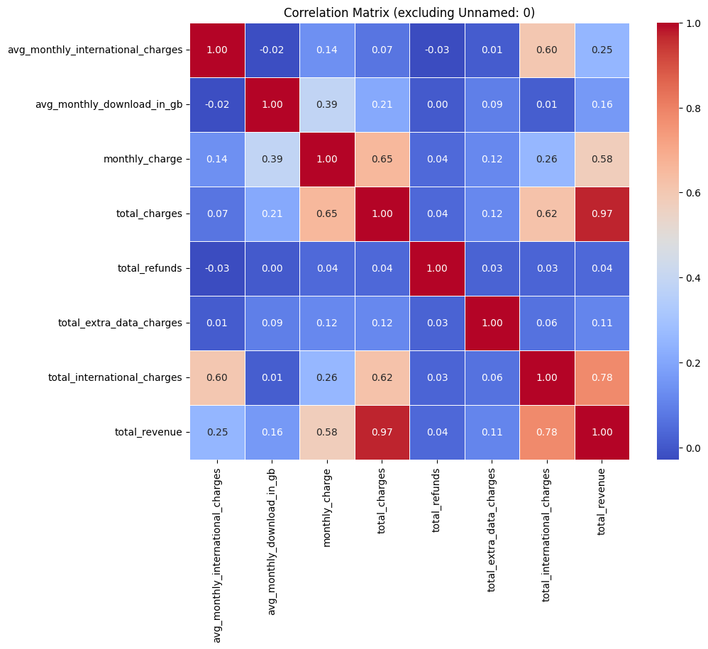
Anomaly detection has no labels, so the discipline is in what you refuse to do. No train/test split, because the job is finding current anomalies in this customer base, not predicting future ones. No handcrafted features, because in an unsupervised task manual feature engineering quietly encodes what the analyst already believes an anomaly looks like. The 82 columns from the merged datasets were cut to 12 by rule: drop one of every pair correlated above 0.8, drop zero-variance columns, drop sparse country dummies. And the contamination setting of 5 percent is written down for what it is, a business assumption about how much abnormal behaviour a base like this can plausibly contain.
Two detectors, one honest choice
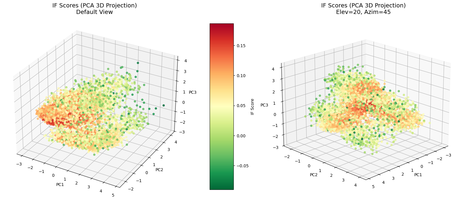
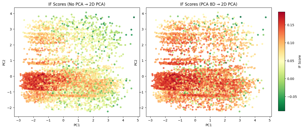
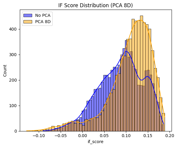
On 7,043 merged customers and the 12 selected features I compared Local Outlier Factor and Isolation Forest, each with and without PCA compression (8 components, chosen because they hold about 80 percent of the variance). No grid search, deliberately: with no labels there is no score to optimise without fooling yourself, so the four configurations were judged on how cleanly they separate the flagged group in projection plots and score distributions. Isolation Forest without PCA separated the anomalies most clearly, and that visible separation is the documented reason it won: the goal here was interpretability, not prediction.
What the anomalies turned out to be
The flagged customers average 13.55 in refunds against 1.33 for normal customers, 55.44 in extra data charges against 4.28, with markedly higher downloads, tenure and referrals. The counterexamples prove the point: customers with refunds of 30, double the anomaly average, still score as normal when their other axes are ordinary. One extreme value is just a heavy user; several at once is a pattern. For a risk team those patterns read as refund policy abuse, referral fraud and missed upsell opportunities, and every flagged case routes to human review before anyone acts on it.
# LOF
lof_model = LocalOutlierFactor(**lof_params)
lof_scores = lof_model.fit_predict(X)
lof_score_values = lof_model.negative_outlier_factor_

# Isolation Forest
if_model = IsolationForest(**if_params)
if_model.fit(X)
if_score_values = if_model.decision_function(X)

X_scores = X.copy()
X_scores['lof_score'] = lof_score_values
X_scores['if_score'] = if_score_values

df_analysis['is_anomaly'] = df_analysis['if_score'] < 0